Interactive Market Correlation Map for Comparing Asset Relationships

Owning more assets doesn't automatically mean a portfolio is diversified: the assets may still move together. An interactive market correlation map shows how asset returns relate, using correlation coefficients from -1 for a perfect inverse relationship to +1 for a perfect positive relationship. A reading near 0 indicates little or no relationship between the returns being compared.

That distinction matters because positive and negative correlations can affect how a mix of holdings behaves. An interactive market correlation map makes relationships easier to compare, but correlation describes past movements, not what assets will do next.

This article explains how to read correlation coefficients, why monthly total returns can help with comparisons, and how positive, negative, or weak relationships can inform diversification. It also explains what a correlation map can and can’t tell you, so you can interpret its patterns without treating them as forecasts.

How correlation relates to portfolio diversification

Correlation measures how asset returns move together, helping investors assess whether different holdings may diversify a portfolio. The result depends on which assets, return data, and time period you compare.

Correlation and Diversification Benefits

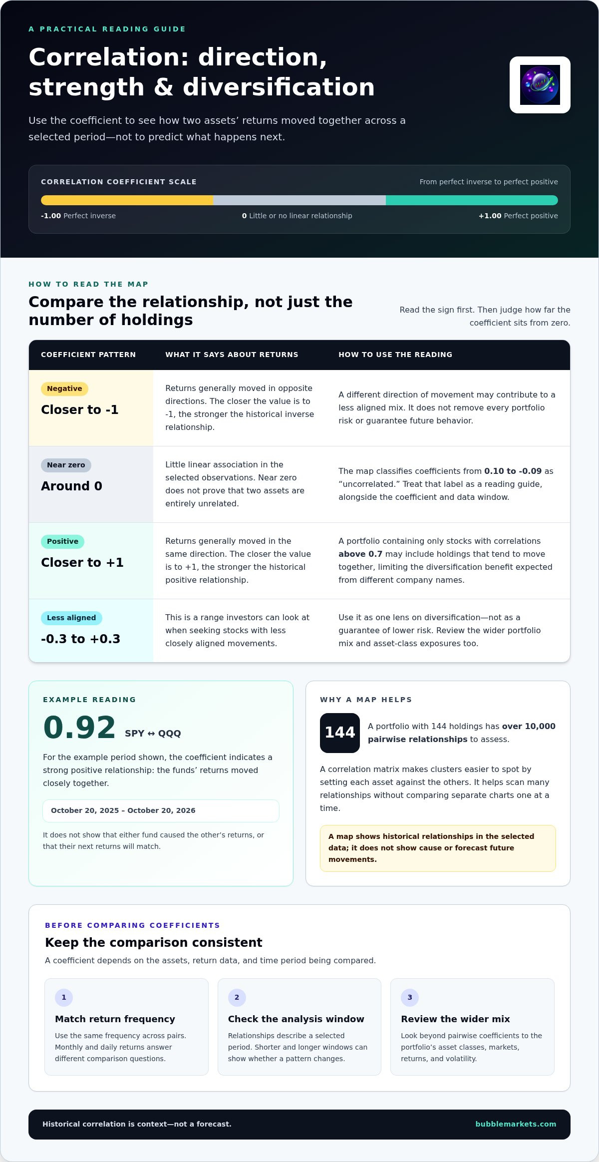
Correlation measures the direction and strength of relationships between asset returns. For diversification, investors can look for stocks with coefficients between -0.3 and 0.3, rather than relying on the number of holdings alone. A portfolio containing 144 holdings has over 10,000 pairwise relationships to assess. A map can make clusters easier to spot, but a low correlation does not remove every portfolio risk.

Comparing Assets Across Markets

Comparing assets across markets means examining return relationships beyond stocks. Market maps may include US Treasuries, non-US stocks, the US dollar, oil, and Bitcoin. To compare stocks, ETFs, currencies, and commodities, use the same analysis window and return frequency, then review each pair’s coefficient. This helps show which assets have moved similarly and which have had less aligned returns.

For US-focused comparisons, the S&P 500 can serve as an anchor for asset-class correlations. A correlation map can show how selected assets, such as US Treasuries or oil, have historically moved relative to that index. Treat the benchmark as a reference point, not a complete view of every relationship in a portfolio.

Correlation Shifts During Market Crises

Correlations describe a selected period, so relationships can differ across market conditions. The market events of 2020 highlighted why portfolio interconnectedness matters: holdings that appeared distinct may respond to shared pressures. Compare shorter and longer windows to see whether a relationship changes across periods. A past pattern is useful context, not a guarantee that assets will move together during the next disruption.

For diversified stock portfolio construction, examine both the pairwise coefficients and the portfolio’s overall mix. A portfolio made up only of stocks with correlations above 0.7 may contain holdings that tend to move together. That concentration can limit the diversification benefit investors expect from holding different company names. Review clusters alongside exposure to asset classes and markets.

Risk management also requires looking beyond correlation. For one example period, October 20, 2025 to October 20, 2026, an equal-weight portfolio had 16.54% volatility, an 18.23% annual return, and a 1.10 Sharpe ratio. Those figures describe that example and period. Use relationship patterns to frame questions about portfolio construction, while assessing returns and volatility separately.

Correlation coefficients and their interpretation

An interactive market correlation map displays coefficients between asset returns, often in a visual matrix. Add or remove assets to tailor the comparison, and use an optional rolling window measured in days, weeks, or months.

Pearson Correlation Coefficients

Pearson correlation measures the direction and strength of a linear relationship between paired returns. Its coefficient summarizes how two investments moved together across the selected observations. Values closer to either end of the scale indicate a stronger linear relationship; a value near zero indicates little linear association.

The calculation standardizes how paired values vary together, making results easier to compare across asset pairs. A correlation matrix sets each asset against the others, letting you review multiple relationships without comparing separate charts one at a time. It describes the selected historical data, not a cause or a future movement.

For example, SPY and QQQ had a displayed coefficient of 0.92 for October 20, 2025 to October 20, 2026. That reading indicates a strong positive relationship across that example period. It does not show that either fund caused the other’s returns, or that their next returns will match.

Reading Correlation Values

A correlation coefficient runs from -1 to 1: 1.00 means perfect positive correlation, 0 means no relationship, and -1 means a perfect inverse relationship. This scale helps readers distinguish assets that have moved similarly from those that have moved in opposite directions. Intermediate values indicate varying degrees of association.

Read the sign first, then how far the value is from zero. A positive value means returns generally moved in the same direction; a negative value means they generally moved in opposite directions. The closer the value is to either endpoint, the stronger the historical relationship. A value near zero indicates little linear association, not proof that the assets are entirely unrelated.

In the displayed example, SPY and QQQ’s 0.92 is close to 1.00, so their returns moved closely together during the selected period. The map also classifies values from 0.10 to -0.09 as uncorrelated. Treat that label as a useful reading guide, then consider the coefficient’s data window and return basis.

For a clear statistical comparison, keep the return frequency consistent across pairs. A coefficient based on monthly returns answers a different question from one based on daily returns. Changing the rolling window can also show whether a relationship shifts over time. Before interpreting a cell, check the assets, frequency, and window.

Monthly total returns used to calculate correlations

For comparisons with the S&P 500, correlations use monthly total returns for each index. Calculation timing follows the selected return interval and rolling window: daily, weekly, or monthly observations produce different comparisons.

A total return includes both price movement and reinvested or paid distributions, where applicable. Using monthly total returns lets each index’s performance be compared over matching calendar periods. For example, compare the S&P 500’s return in one month with another index’s return for that same month, then repeat across the selected window.

Matching periods matters because each correlation pairs returns from the same dates. If one asset’s return for a period is matched with another asset’s return from a different period, the result no longer describes movement over aligned intervals. Before reading a visualization, confirm that the return basis, assets, and window match the comparison you want to make.

Daily, weekly, and monthly intervals answer different questions. Daily returns capture shorter moves and can react quickly to market events; weekly returns group those moves into broader periods. Monthly returns smooth the view across each month, which is the basis used for the S&P 500 asset-class comparison. A coefficient can differ across intervals because the paired observations differ.

Annual returns help review performance over full-year periods, but provide fewer observations than monthly returns across the same span. Monthly analysis shows relationships across individual months, while annual figures summarize each year. Choose the interval that fits your question, and don’t treat an annual relationship as interchangeable with a monthly one.

How often are correlation calculations updated? They follow the selected frequency and analysis window. A daily basis uses daily returns; a monthly basis uses monthly total returns. As the rolling window advances or changes length, the observations in the calculation change too. The interval sets the pace of the comparison, while the window determines which historical periods it covers.

For a practical check, compare the same two indexes using daily, weekly, and monthly returns, then see whether the relationship remains similar. A difference between daily and monthly coefficients reflects different observation intervals, not necessarily an error. Keep the interval consistent when comparing several pairs in a matrix, and note the window alongside each result.

Monthly total returns provide a consistent basis for comparing index performance across matching months. They don’t capture every short-term move, while annual returns compress more information into fewer observations. Check both the interval and window to understand what the correlation measures before using it in an investment decision.

Correlation ranges categorized as high, moderate, or low

Range labels offer a quick visual cue, but their thresholds depend on the map’s classification scheme. Read the coefficient and its sign alongside the label, then consider how the historical relationship applies to your comparison.

One map classifies positive correlations from 0.7 to 1.0 as high, from 0.4 to 0.7 as moderate, and from 0.0 to 0.4 as low. For negative correlations, it labels (0.7) to (1.0) high, (0.4) to (0.7) moderate, and (0.0) to (0.4) low. Parentheses here indicate negative values.

These bands help scan a matrix: a high positive reading suggests assets historically moved closely in the same direction, while a high negative reading indicates a strong inverse relationship. A low band signals a weaker relationship. For example, a coefficient of 0.92 falls in the high positive range, while a value near zero falls within the low range.

• High positive: 0.7 to 1.0, indicating closely aligned movement.
• Moderate positive: 0.4 to 0.7, indicating a less pronounced positive relationship.
• Low: 0.0 to 0.4 on the positive side, or (0.0) to (0.4) on the negative side.
• Moderate negative: (0.4) to (0.7), indicating an inverse relationship.
• High negative: (0.7) to (1.0), indicating a stronger inverse relationship.

Classification systems don’t always use identical cutoffs. Another tool labels 1.00 to 0.51 as strong positive, 0.50 to 0.11 as moderate, 0.10 to -0.40 as weak inverse, and 0.41 to -1.00 as strong inverse. Those labels differ from the ranges above, so don’t combine both schemes as if they were one standard.

Boundary values also need care. The first scheme includes 0.7 as the endpoint for both high and moderate positive ranges, and (0.7) for both negative ranges. If a coefficient sits on a shared boundary, use the map’s displayed label and inspect the actual value. The label is a category, not a replacement for the coefficient.

Use categories to prioritize comparisons, not to decide based on color alone. First identify whether the coefficient is positive or negative, then note its magnitude, classification scheme, and historical period. A moderate or low label summarizes the selected data. It doesn’t explain why assets moved together or predict their next relationship.

The study describes reducing high-dimensional data to a 2-dimensional surface for visualization. Multidimensional scaling projects high-dimensional data into two or three dimensions while preserving pairwise distances.

Interpreting positive and negative correlations

A positive coefficient means two assets have historically tended to move in the same direction; a negative coefficient means they have tended to move in opposite directions. The sign shows direction, while the distance from zero indicates the strength of the measured relationship. Consider both when assessing how a pair may contribute to portfolio diversification.

At +1, returns have a perfect positive relationship; at -1, they have a perfect inverse relationship. A coefficient near zero signals little linear relationship over the analyzed period. These readings describe paired historical returns, not asset quality, likely future performance, or the size of future gains and losses.

Positive correlation can concentrate exposure. If several assets rise and fall together, holding them together may provide less diversification than their different names suggest. A high positive coefficient, such as a value in the map’s 0.7 to 1.0 range, flags a relationship worth examining alongside each holding’s role and portfolio weight.

Negative correlation describes a different pattern: one asset’s returns have tended to move against another’s. That may help offset some portfolio fluctuations, but the coefficient alone doesn’t show how much volatility the mix will experience. Consider the relationship alongside each asset’s weight, return history, and contribution to overall portfolio movement.

Three distinctions help prevent overreading a map:

• Direction: A positive sign indicates same-direction movement; a negative sign indicates opposite movement.
• Strength: Values nearer +1 or -1 indicate a stronger historical relationship than values near zero.
• Scope: The coefficient applies to the selected assets, return basis, and analysis window, not every market condition.

For example, an asset pair with a negative coefficient may still lose value at the same time. An inverse relationship means returns tended to move in opposite directions across the observations, not that one asset reliably protects the other. Similarly, a low coefficient doesn’t mean an asset has low volatility; it describes the relationship between two return series.

Use an interactive market correlation map to spot clusters and contrasts, then inspect the coefficients. Compare the same pairs across different historical windows: a relationship can weaken, strengthen, or change direction as the selected period shifts. This helps distinguish a persistent pattern from one specific to the chosen window.

For a focused review, select a pair, note its sign and magnitude, and compare that reading with the portfolio’s existing exposures. Then examine whether the relationship changes across the displayed periods. Compare asset relationships in market maps to inspect positive and negative patterns across selected markets.

BubbleMarkets: Free Live Market Bubble Maps

BubbleMarkets offers free live market bubble maps for visual market scanning, as well as focused stock and crypto bubble maps. Use these views to compare market activity visually, then apply the correlation concepts above to interpret historical relationships between asset returns. Pro, Professional, and Enterprise subscriptions provide additional options, including advanced visualization tools and extended screening. Bubble maps show market activity visually; correlation analysis is a separate way to assess how asset returns have moved together.

Explore BubbleMarkets’ maps to find a view that suits the market you’re examining. Visit bubblemarkets.com to explore the available market maps.

Make Your Next Comparison More Focused

Before opening an interactive market correlation map, define your question: are you examining overlap between holdings or relationships across asset classes? A clear comparison helps you choose which assets and time window to inspect. Record what you want to understand and how the observed relationship informs your portfolio review. This keeps the analysis tied to a decision rather than turning a visual pattern into a conclusion on its own.

Use the map as one input alongside your own investment criteria. Historical relationships can help frame a comparison, but they don’t replace your assessment of exposure, volatility, and objectives. Next, choose a market view that fits your analysis and explore how it can support your workflow.

Contact BubbleMarkets to discuss your needs and find a suitable starting point for your market comparisons. A focused question makes the data easier to examine and your next review more purposeful.

Frequently Asked Questions

What is stock correlation and why does it matter?

Stock correlation describes how the returns of two stocks have related over a selected period. It can help distinguish overlapping exposures from relationships that may behave differently. For example, two companies in separate industries can still have similar historical movements, while stocks in the same industry may diverge. Compare the coefficient with your portfolio’s existing holdings. It adds context, but doesn’t determine whether either stock suits your goals.

What's the difference between daily, weekly, and monthly correlations?

Daily, weekly, and monthly correlations group returns at different intervals, so the same assets can show different patterns. Daily data can reveal short-lived market moves; weekly and monthly views group those fluctuations into broader comparisons. If you’re evaluating a long-term allocation, a monthly view may better match that horizon. For a short-term review, compare shorter intervals without assuming they predict the next move.

How is market correlation calculated, and what time periods are used?

Market correlation is commonly calculated using Pearson correlation on paired returns for two assets. The calculation compares how the return series vary together across matching observations. Depending on the question and available window, analysis can use daily, weekly, or monthly returns. For a meaningful comparison, keep the return interval consistent across asset pairs and note whether the calculation uses a fixed historical period or a rolling window.

Which platforms offer interactive market correlation maps?

BubbleMarkets offers visual market maps across asset classes, including ETFs, commodities, forex, bonds, and world indices, as well as stock and crypto views. Market screeners and heat maps provide additional ways to scan market data. These tools support visualization and comparison; they aren’t brokerage services or personalized investment advice. Choose a view based on the assets you want to examine and whether you need a broad market scan or a focused asset-class comparison.

What are the limitations and risks of using correlation data for trading?

Correlation data can mislead when a historical relationship is treated as a trading signal. A pair can have low correlation while both assets remain volatile, and a previously negative relationship can change as market conditions shift. The coefficient also doesn’t explain why returns moved together. Before using a reading in a trading decision, consider the selected window, each asset’s separate risk, and whether the relationship fits your wider analysis.